10 Excel Formulas for Non-Excel Users

Microsoft Excel is without a doubt the most powerful spreadsheet among those who work in an office; accountants, bookkeepers, data entry clerks, and all types of administrators. The environment that it offers may not be as user-friendly as other software, but If you have access to MS Office and have a plan to analyze your work, at least some of the very basic formulas will become essential. It's not as complicated as a programming code, you just have to remember how each syntax should be laid out.

Other spreadsheets such as Google Sheets and Apple Numbers do not have as many formulas as Excel because they are primarily designed for individuals, not for professionals. However, some basic formulas are indeed useful for you to manage home finance or data entry. If you want to create an inventory of thousands of books that you have, for example, the formulas will help you sort, categorize, total purchase price by category, etc. Knowing the fundamentals of formulas is enough to get started.

1. IF Statements

The IF function is used to check for a specific condition in the data. It is a helpful function to organize and detect any specific condition that you want.

Let’s see a simple example to understand how the IF function works. 

=IF(logical_test, [value_if_true], [value_if_false])

Logical_test:Refers to the specific condition that you want to check

Value_if_true: Refers to the returned value if the condition matches

Value_if_false: Refers to the returned value if the condition does not match

In this example, we used the IF function to return “Yes” where a product is “Red” and return “No” if the color is not red. 

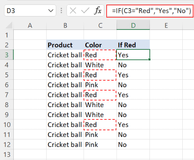
From the above screenshot, the words "red", "white", "pink" may look simple enough. But when a list has thousands of items and the words are similar or complicated, IF statement becomes useful. You can also use COUNTIF to check the number of Yes/No, which will be extremely handy when you have a lengthy list.

Alternative in Google Sheets

If you want to use Google sheets, it also provides the IF function with the same structure. You can follow the above instructions in Google sheets to use the IF function.

2. SUM and SUMIF

The sum is a function that is used to perform a simple sum operation on the numerical values in Excel.

=SUM(number1, number2,…..

Number1,2,…Refers to the numerical value(s) that are to be summed up

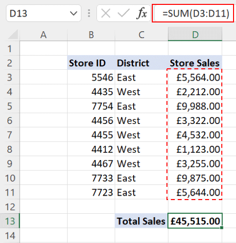
Below is a simple example using the SUM function where individual store sales are summed up. 

The SUMIF function is a bit more advanced but offers more flexibility. It allows you to sum the values based on specific criteria.

=SUMIF(range, criteria, [sum_range])

Range: Refers to the range where the condition will be searched

Criteria: Refers to the actual condition to be used

Sum_range: [Optional] Refers to the actual range of values to be summed up. It is required when criteria and sum range are not the same.

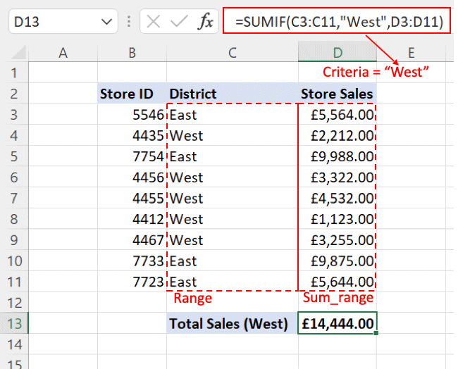
Let’s revisit the above example, but now we want to sum up the sales values of stores that are situated in the West district only.

To do that, SUMIF can be used by assigning the “District” column as Range, defining “West” as our Criteria, and the “Store Sales” column as our Sum_range.

 Alternative in Google Sheets

Google sheets also offers the SUM and SUMIF functions. The arguments for both functions are also the same as in Excel. 

3. COUNT and COUNTIF

The COUNT function is used to count the number of occurrences of numerical values in a range. 

Numerical values in Excel includes negative numbers, date, times, percentages, fractions, and formulas that return numbers.

=COUNT(value1,[value2],…)

Value1,2,..:Refers to the values that are to be counted. A range can also be defined in it

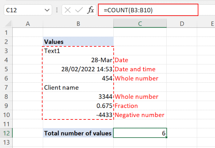
Suppose you want to count the numerical values occurring in a range of mixed data types, you can use the COUNT function. Refer to the below example.

The COUNTIF function enables you to count the values based on specific criteria. Besides numerical values, the COUNTIF function can also be used for textual data.

You can define the condition in the COUNTIF function by using logical operators like (<, >, = or <>)

=COUNTIF(range, criteria)

Range:Refers to the range containing values to be counted

Criteria:Refers to the specific condition that is to be counted

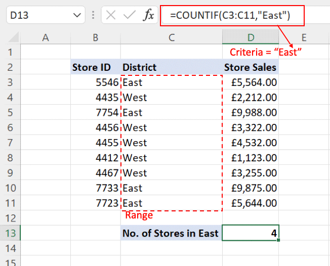
In the example below we are counting entries where the district is “East”.

Alternative in Google Sheets

Both COUNT and COUNTIF functions are available in Google Sheets with similar arguments. You can try using both functions by recreating the above examples in Google Sheets. 

4. XLOOKUP

XLOOKUP function is among the latest functions that Excel has rolled out in Microsoft 365 and later versions of Excel.

It is helpful to look up information from multiple workbooks and within the same workbook. 

XLOOKUP is the improved function that can easily replace all the existing look-up functions like VLOOKUP, HLOOKUP, and LOOKUP.

=XLOOKUP(lookup_value, lookup_array, return_array, [if_not_found], [match_mode], [search_mode])

Lookup_value:Refers to the required value that is to be looked up from the data

Lookup_array:Refers to range of values containing the target value

Return_array:Refers to the range containing the returned value(s)

If_not_found:Optional; Refers to the returned value if the required value is not found

Match_mode:Optional; 0 = exact match (by default), -1 = exact or next closest match, 1 = exact or next larger match, 2 = wildcard entries

Search_mode:Optional; 1 = search from the first value (default), -1 search from the last value

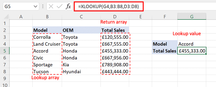
Refer to the below example of using XLOOKUP.

Alternative in Google Sheets

Currently, Google Sheets does not offer the XLOOKUP function. To look up values in Sheets, you need to use the VLOOKUP, HLOOKUP functions. These functions will be enough for the basic lookup requirement.

However, for more advanced look-up requirements, you can use the combination of INDEX and MATCH or INDEX and SEARCH functions.

5. AND

AND is a logical operator that is used to check two or more conditions at the same time. It is helpful when you need to validate values based on multiple criteria.

It will return TRUE when all the conditions entered are met and return FALSE even when the condition is not met one or more times. 

=AND(logical1, logical2,…)

Logical1,2,…:Refers to the expression that you want to use

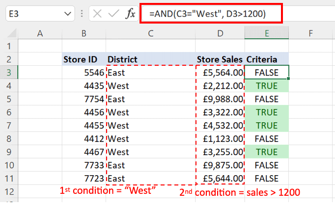
Refer to the below example to understand the AND function:

Here, we are trying to find out stores that are in the “West” district (Condition 1) and have sales of more than £1200 (Condition 2). Where both conditions have been met, Excel has returned TRUE in the column named “Criteria”.

Alternative in Google Sheets

AND function is also available in Google Sheets with the same structure as stated above.

Also Read: 10 Kickass Google Sheets Templates to Improve Your Website’s SEO

6. NOW

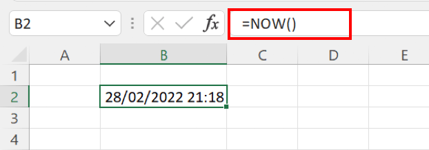
NOW function returns the current date and time. The value returned by the function keeps on updates each time the worksheet is opened.

The NOW function takes no argument inside the parenthesis.

=NOW()

Alternative in Google Sheets

NOW function is also available in Google Sheets having the same structure as stated above.

7. CONCATENATE

The CONCATENATE function in Excel joins several strings of text from different cells into one combined string of text. 

=CONCATENATE(text1,text2,….)

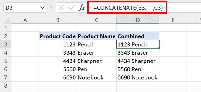
Notice in the above screenshot that there's " " (quotation marks) in between B3 and C3 - that's a space. Without the quotation marks with a space in between, it will be displayed as 1123Pencil. You will insert " " so that you may want the combined display to show as 1123 Pencil.

Alternative in Google Sheets

Google Sheets also offer the CONCATENATE function with the same formula structure.

8. LEFT RIGHT and MID

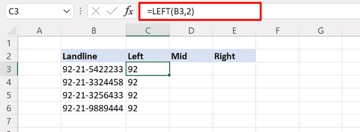
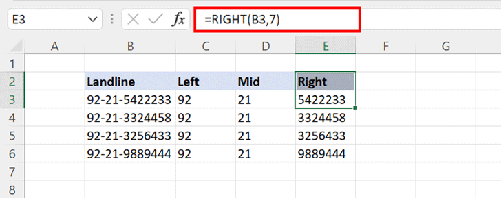
These are useful formulas to work with textual data. You can extract the required amount of characters by applying these formulas from the a text string.

Function arguments for LEFT and RIGHT are the same, while MID is a bit different.

=LEFT(text, [num_chars])

Text:Actual text from which the characters are to be extracted

Num_chars:Number of characters required to be extracted

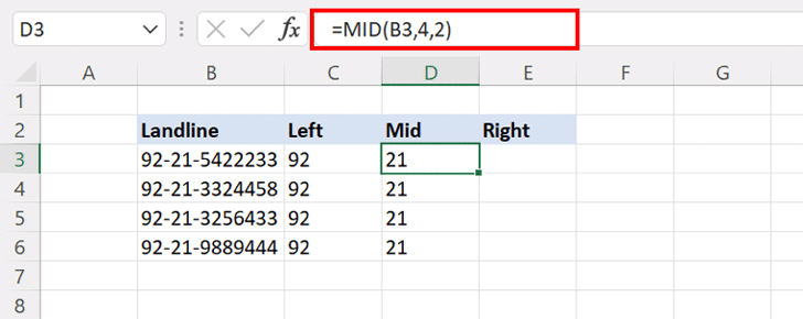
=MID(text, start_num, num_chars)

Text:Actual text from which the characters are to be extracted

Start_num:The starting point to extract the characters (counting from the left)

Num_chars:Number of characters to be extracted

Alternative in Google Sheets

LEFT, RIGHT, and MID functions are also available in Google Sheets.

9. MAX and MIN

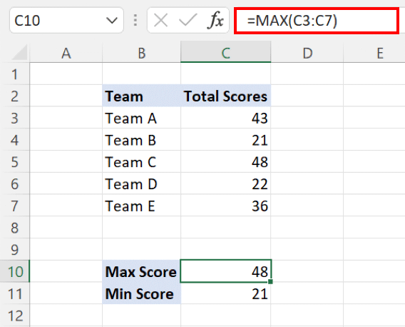
MAX and MIN functions in Excel help you to quickly identify the largest and smallest values from a range of numbers.

Both functions are easy to use and require a range of values as an argument.

=MAX(number1,number2,…)

Alternative in Google Sheets

Both MIN and MAX functions are available in Google Sheets having a similar formula structure

10. PROPER

PROPER is a useful function to work with textual data. It gives the proper structure to the text string by capitalizing the first letter of each word.

=PROPER(text)

Text:Text string to be converted into the proper structure

Alternative in Google Sheets

PROPER function is available in Google Sheets and can be used similarly as described above.

Final Thoughts

The above 10 are some of the absolute basic formulas that Microsoft Excel can do for you. If you’ve had no previous knowledge, I hope the information can at least help you get the feel of it. Google Sheets are available for every Google user for free, so you can easily replicate these formulas without spending money on Microsoft Office.

If you are interested in learning a lot more powerful calculation functions, Excel actually has hundreds of more formulas; some simple, some mindbogglingly complicated, and you can also create a nested formula by mixing two or more formulas. These are the reason Excel is seen as one of the most essential tools among professionals who require all sorts of business analysis.